A frequentist approach to prediction uncertainty
Uncertainty for single predictions becomes more and more important in machine learning and is often a requirement at clients. Especially when the consequenses of a wrong prediction are high, you need to know what the probability (distribution) of an individual prediction is. In order to calculate this, you probably think about using Bayesian methods. But, these methods also have their downsides. For example, it can be computationally expensive when dealing with large amounts of data or lots of parameters. What I didn’t know was that you actually can get similar results using frequentist methods. This post will explain how you can calculate different types of uncertainty for regression problems using quantile regression and Monte Carlo dropout. All code used in this blog will be published on Github.
Uncertainty
In order to calculate the uncertainty, you need to distinguish the type of uncertainty. You can define many different types of uncertainty, but I like the distinction between aleatoric and epistemic uncertainty. Aleatoric (also referred to aleatory) uncertainty is uncertainty in the data and epistemic uncertainty is the uncertainty in your model. With model uncertainty I do not mean uncertainty about the modelling approach. The decision between a LinearRegression or RandomForestRegressor model for example is still up to you.
The toy dataset
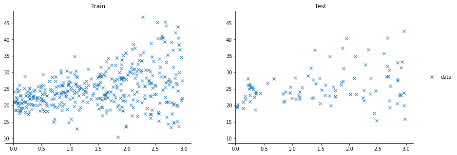
For the next examples, we’ll use a toy dataset with two variables, $x$ and $y$, to make sure we can easily understand/visualize what is happening. The dataset looks like this:
Aleatoric uncertainty
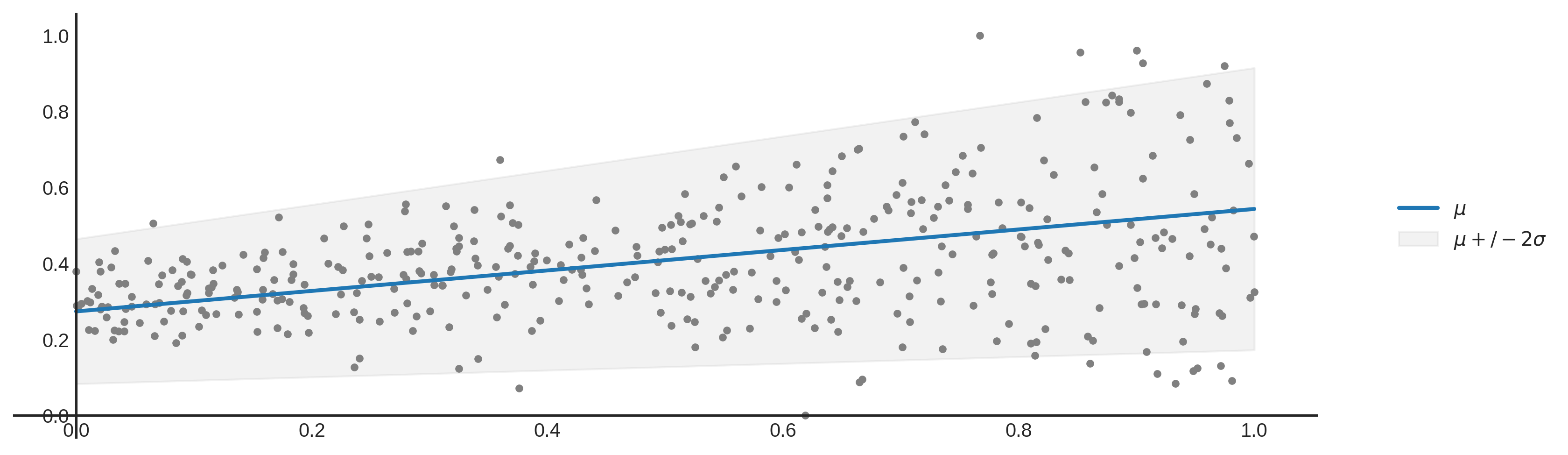
Aleatoric uncertainty (or statistical uncertainty) is the uncertainty in your data. This can be uncertainty caused by errors in measuring the data, or by the variability in the data. With variability in the data I mean the following. Lets say that you have one input feature being house area to predict the house price. It is very likely that there are different house prices in the data set with the same house area. This variance in the house price is defined as aleatoric uncertainty. In our plot above, the aleatoric uncertainty is equal to the mean plus or minus 2 times the standard deviation.
Epistemic uncertainty

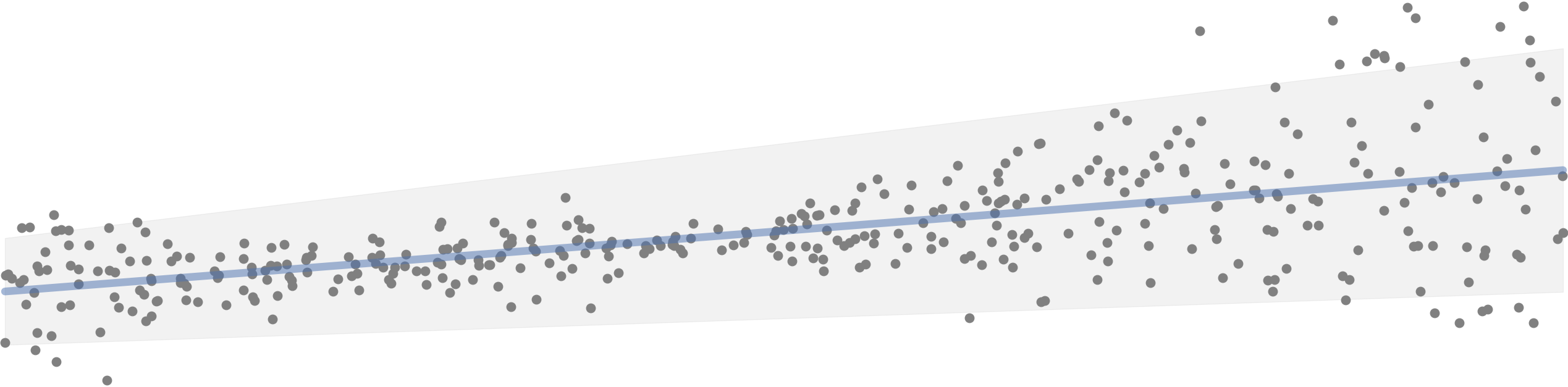
Epistemic uncertainty (or systematic uncertainty) is the uncertainty in the model. You can interpret this uncertainty as uncertainty due to a lack of knowledge. For example, I am uncertain about the number of people living in the Netherlands, but this information can be obtained. In data science epistemic uncertainty can be reduced by improving the model. In our example plotted above you can say that all lines fit the data reasonably well, but which line fits the data the best? Using linear models from SKlearn for example, we choose a model that performs best for a certain metric (global or local optimum) and ignore the epistemic uncertainty.
Modelling uncertainty
Now we know what types of uncertainty we have to deal with. To model these different uncertainties, we use two different techniques called quantile regression and Monte Carlo Dropout [2]. When we have calculated both uncertainties, we can sample and approximate the posterior predictive distribution. Lets start with quantile regression.
Quantile Regression
When you read this, I expect you know linear regression. When using L2 regression (regular OLS), we minimise the squarred error. When using L1 regression (or LAD regression) we minimise the absolute error. Quantile regression is very similar to L1 regression. When fitting quantile 0.5 ($\tau=0.5, \tau\in[0,1]$) also known as the median, Quantile Regression and LAD regression are even the same. The difference is in the symmetry of the loss function. Quantile loss (or pinball loss) can for example also be assymmetrical. Quantile loss is defined as:
\[L_{t}= \begin{cases} (y - \hat{y})\tau, & \text{if } y\geq\hat{y} \\\\\\ (\hat{y} - y)(1 - \tau), & \text{otherwise} \end{cases}\]When changing $\tau$ the loss function changes and starts to treat under and over prediction differently. Take a look at the following plot:
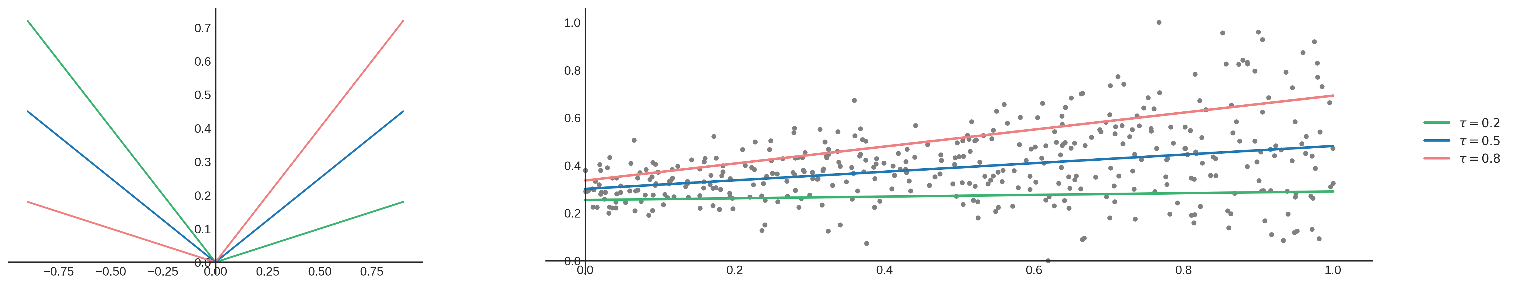
The blue line has a symmetrical quantile loss function for $\tau=0.5$. Positive and negative errors are treated equally, which results in a linear function that fits the median. When choosing a different $\tau$, for example $\tau=0.2$, the loss function changes and the line fits a to a lower part of your data as you can see by looking at the green line. This is because the error function gives a higher penalty to underprediction compared to over prediction (positive error curve is less steep than the negative error curve). For a higher $\tau=0.8$ it is the other way around as shown by the red line.
Another nice property of fitting quantiles is that we don’t have an error distribution assumption, which OLS for example does have.
Multiple quantile regression
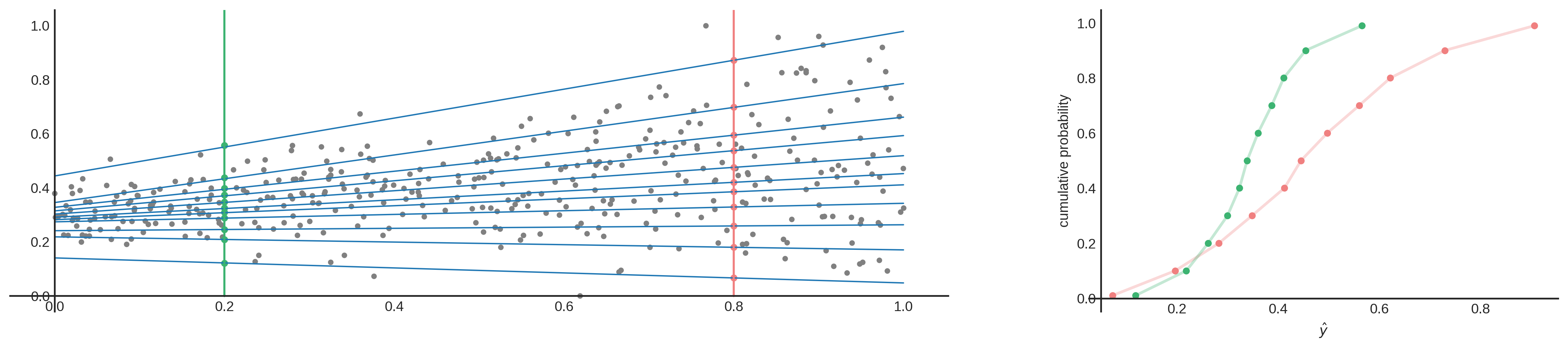
So why do we need this? Quantile regression allows us to fit lines to different parts of the data. These parts are not just parts, but have meaning as well. To explain this, I’ll start again with the median ($\tau=0.5$). The property of the median is that it is the middle value of your data. You can expect that ~50% of the data lies above this point, and the other half below. So when you fit a line to the median of your data, you can assume the same about your prediction. This holds for other quantiles as well. Quantile regression for $\tau=0.8$, means that we expect that 80% of the data lies below the line. You can also interpret it like this: I’m 80% sure that the true value is equal to $\hat{y_{\tau}}=0.8$ or lower. Or, I’m 60% sure that the true value is between $\hat{y_{\tau}}=0.2$ and $\hat{y_{\tau}}=0.8$. These scentences sound familiar right? When you have a Cumulative Distribution Function (CDF), you can get these types of conclusions. Therefore, by using multiple quantile regressions, you can estimate points on a CDF. When you fit enought quantile regression lines, you can approximate a CDF (as shown below) and calculate aleatoric uncertainty!
To build this multiple quantile regression, you can use Statsmodels’ QuantReg and manually fit multiple quantiles. You could also use XGBoost to do this, as explained in this blog. You can even use SKlearn’s RandomForestRegressor as explained here. And of course, you can use deep learning as well since we can simply implement the quantile loss function (eq. 1) to train our neural net. This last option is the one I’ll be using since it’s fast and it performs well. Here you can see my implementation in PyTorch:
from functools import partial
import torch
from torch import nn
import numpy as np

def QuantileLoss(preds, target, quantiles):
    def _tilted_loss(q, e):
        return torch.max((q-1) * e, q * e).unsqueeze(1)

    err = target - preds
    losses = [_tilted_loss(q, err[:, i])  # calculate per quantile
              for i, q in enumerate(quantiles)]

    loss = torch.mean(torch.sum(torch.cat(losses, dim=1), dim=1))
    return loss

class DeepQuantileRegression(nn.Module):
    def __init__(self, params):
        super().__init__()
        self.hidden_size = params['hidden_size']
        self.quantiles = params['quantiles']
        self.model = nn.Sequential(
            nn.Linear(params['input_size'], params['hidden_size']),
            nn.Linear(params['hidden_size'], len(params['quantiles']))
        )

    def forward(self, X):
        return self.model(X)

QUANTILES = np.array([.01, .1, .2, .3, .4, .5, .6, .7, .8, .9, .99])
params = {
    'input_size': 1,
    'hidden_size': 128,
    'dropout_p': 0.2,
    'dropout_dim': 1,
    'quantiles': QUANTILES,
    'batch_size': 16,
    'epochs': 200,
    'lr': 1e-4,
    'weight_decay': 1e-6,
}
model = DeepQuantileRegression(params)
optimizer = torch.optim.Adam(model.parameters(),
                             lr=params['lr'],
                             weight_decay=params['weight_decay'])
criterion = partial(QuantileLoss, quantiles=QUANTILES)
Here you can see that by simply making a neural net with some arbitrary number of output accompanied by a quantile loss function you can model aleatoric uncertainty. One thing to mention, or better, to watch out for, is called quantile crossover. When fitting multiple quantile regressions it is possible that individual quantile regression lines over-lap, or in other words, a quantile regression line fitted to a lower quantile predicts higher that a line fitted to a higher quantile. If this occurs for a certain prediction, the output distribution is invalid. This especially happens when you are fitting your quantiles independently. In our architecture we fit the quantiles together at the same time, which is called composite quantile regression. This helps to fit the quantiles better and reduces quantile crossover, but doesn’t guarantee non-crossing regression quantiles. There are methods that guarantee non-crossing quantiles, which require a more complex implementation[2]. I will try to dig deeper into these monotonicity constraints to see how this can be guaranteed. In my experience, when manually evaluating the cases where quantile crossover occurs, I could often find weird input features causing this. For me this was an indicator that my preprocessing missed something, or that there are some quirks in the data.
This deep learning approach allows us to do one other thing, which is called Monte Carlo Dropout. This allows us to model epistemic uncertainty as well.
Monte Carlo Dropout
Dropout is a technique used in deep learning to regularize the model and reduce overfitting. Normally dropout is only used during training, and (automatically) turned off during inference. In 2015, Yarin Gal and Zoubin Ghahramani introduced a way of using dropout in (deep) neural networks as approximate Bayesian inference in deep Gaussian processes[3]. Which I would translate into: they show that using dropout during inference allows you to obtain (epistemic) uncertainty. To do this, you need to make sure that dropout is implemented before every hidden layer and applied during inference. Then you need to predict multiple times (e.g. 1000 times) for each set of input features. If you do this many times, you get a distribution of values for an individual prediction instead of 1 single value. Intuitively you can see it like this.
Every time you do a forward pass, some hidden states are masked out. This results in a slightly different network architecture every time you do a prediction. And if you repeat this many times, you have many slightly different models, predicting different values. The wider this distribution is, the less certain the model is about a certain output, and vice versa. Implementation wise, it was a bit more tricky to implement this. The regular dropout layer, nn.Dropout(), creates a 2d (batch_size, hidden_size) matrix with random 1’s and 0’s based on the dropout probability p. This means that every set of hidden features in your batch, gets different hidden features masked out. Normally, this shouldn’t be a problem and is actually computationally cheaper to do. But, since I’m trying to create a linear quantile regression line, the dropout mask used in a single batch must be equal for all sets of hidden features in that batch. You can see it as a dropout mask that is based on 1 set of hidden features, and then broadcasted over all sets of hidden features in the same batch. You can try it for yourself using the regular nn.Dropout() layer. You’ll see that the output is no longer linear. In your neural network architecture dropout must be applied before every hidden layer. Here you can see my implementation in PyTorch and update of the model architecture.
import torch
from torch import nn
import numpy as np

class Dropout_on_dim(nn.modules.dropout._DropoutNd):
    """ Dropout that creates a mask based on 1 single input, and broadcasts
    this mask accross the batch
    """
    def __init__(self, p, dim=1, **kwargs):
        super().__init__(p, **kwargs)
        self.dropout_dim = dim
        self.multiplier = 1.0 / (1.0-self.p)

    def forward(self, X):
        mask = torch.bernoulli(X.new(X.size(self.dropout_dim)).fill_(1-self.p))
        return X * mask * self.multiplier

class DeepQuantileRegression(nn.Module):
    def __init__(self, params):
        super().__init__()
        self.hidden_size = params['hidden_size']
        self.quantiles = params['quantiles']
        self.model = nn.Sequential(
            nn.Linear(params['input_size'], params['hidden_size']),
            Dropout_on_dim(params['dropout_p'], dim=params['dropout_dim']),
            nn.Linear(params['hidden_size'], len(params['quantiles']))
        )

    def forward(self, X):
        return self.model(X)

    def mc_predict(self, X, samples=4000):
        with torch.no_grad():
            self.model.train()
            preds = np.array([self.model(x_train).numpy().T for _ in range(samples)])
        # To return shape: batch_size, n_quantiles, samples
        return np.swapaxes(preds, 0, -1)
Approximate predictive posterior distribution
Now, per individual prediction, we have many different CDFs. Each CDF represents the aleatoric uncertainty and is created using quantile regression. All (slightly different) CDFs represent the epistemic uncertainty which are generated using Monte Carlo dropout. In order to get the approximate predictive posterior distribution, we need to combine all CDFs into a single distribution. To do this, we uniformly sample a floating number between 0 and 1, to represent a random quantile. Also, we don’t have a distribution function. We only have a few (11 in this case) point estimates of that distribution. Therefore, we interpolate the corresponding $\hat{y}$ of each CDF. You can easily implement this using Scipy’s interpolate module.
from scipy.interpolate import interp1d

def get_quantile_pred(q, used_quantiles, preds):
    interp_cdf = interp1d(used_quantiles, preds, fill_value='extrapolate')
    return interp_cdf(q)
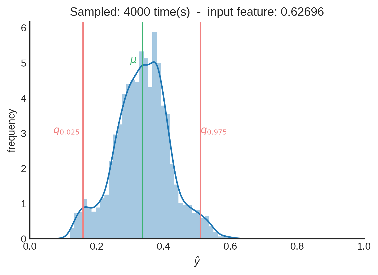
When we combine many of those samples, we approximate the predictive posterior distribution that represents both aleatoric and epistemic uncertainty.
After 4000 samples in this case, we can say that the the mean of the distribution ($\mu≈0.33712$) is a good point estimate. When you want to be 95% sure, you can state that the true value is between $0.15950$ and $0.51058$. You can see this interval as the credible interval.
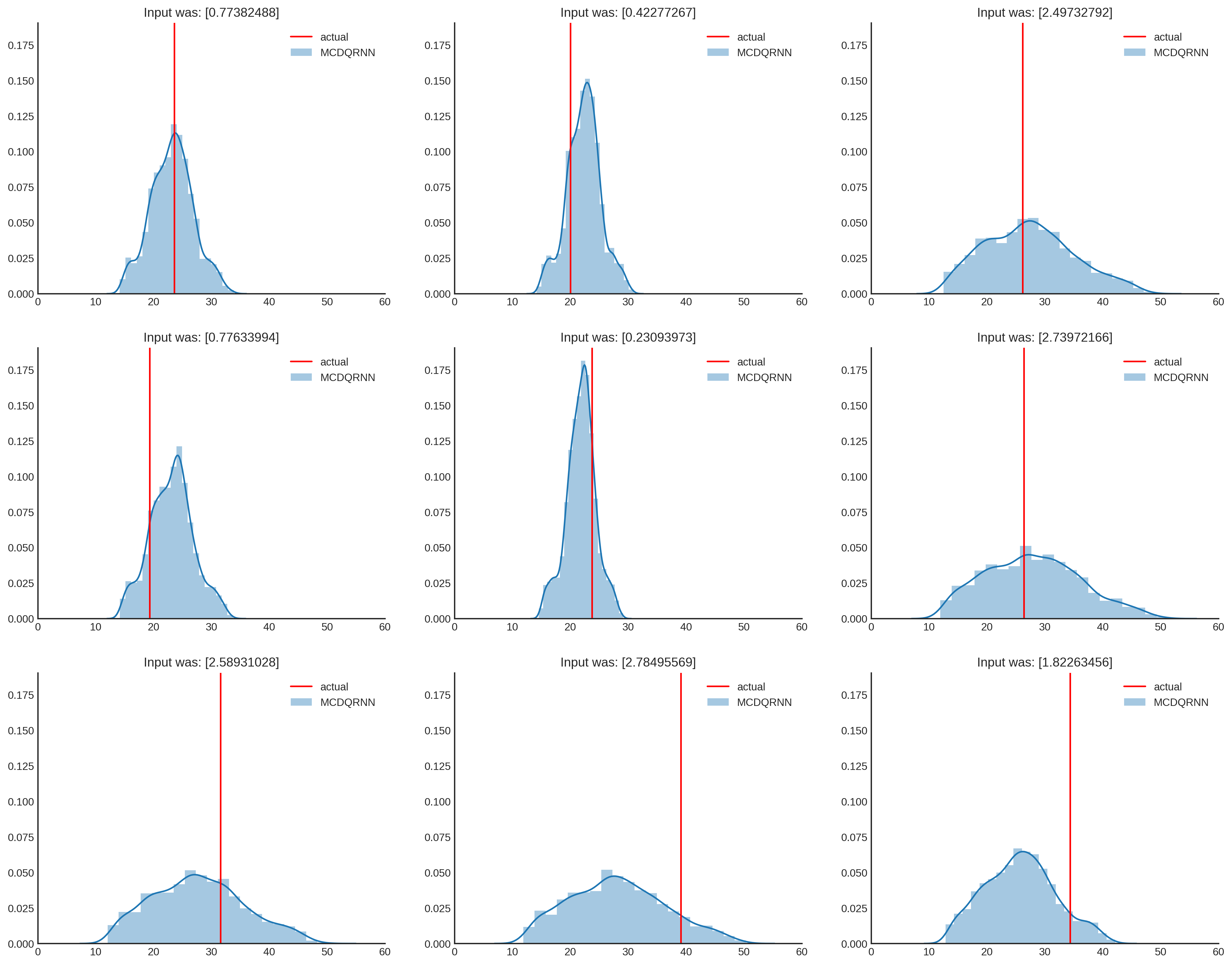
And one last side note, since Quantile regression has no (error) distribution assumption, the outcome doesn’t have to be normally distributed. As shown below, the distribution can get different shapes and quantify different levels of uncertainty. As $x$ becomes higher, the uncertainty increases, which seems fair when looking at the data. And that’s it, we have modeled prediction uncertainty!
.
Discussion
In this example, the dropout rate had a big impact on the uncertainty and training process. Mainly because a prediction depends on only one input feature and if that information is (partially) dropped out, it is more difficult to make a good prediction. In a more real-life use case you normally have more input features, which will probably make the predictions more stable. I am planning to use this architecture on a public dataset to compare / review the performance. Another thing I would like to try is predicting a mean $\mu$ and standard deviation $\sigma$ instead of using quantile regression, while still using MCDropout. Lots of new things to try I guess!
References
[1] https://en.wikipedia.org/wiki/Uncertainty_quantification
[2] Alex, J. Cannon, Non-crossing nonlinear regression quantiles by monotone compositequantile regression neural network, with application to rainfallextremes, https://link.springer.com/content/pdf/10.1007%2Fs00477-018-1573-6.pdf
[3] Yarin Gal, Zoubin Ghahramani, Dropout as a Bayesian Approximation: Representing Model Uncertainty in Deep Learning, https://arxiv.org/pdf/1506.02142.pdf