Prediction uncertainty part 2

In this post, I would like to continue where I left off in the previous post regarding prediction uncertainty by showing a second frequentist way of calculating uncertainty for regression problems. After fitting the quantiles (aleatoric uncertainty) and sampling using MCDropout (epistemic uncertainty), we combined the sampled distributions in a single distribution. We did this by sampling from each sampled CDF. This CDF however, wasn’t a full distribution but a collection of quantile predictions. In order to sample from it, we used linear interpolation in between the quantile predictions. Nothing wrong with that, but I wanted to see if there was an easier way to combine the distributions into a single predictive posterior distribution. In this blog post I’ll explain another way to calculate and combine aleatoric and epistemic uncertainty. All code used in this blog will be published on Github. In first notebooks you will find a more elaborate explaination of the code. In the next notebooks, as well as in the package, I’ve wrapped the model classes in a SKlearn-like interface. This allows me to create cleaner notebooks in the comparison phase.

The data

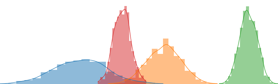
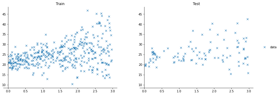
Like last time, we’re using a generated dataset, that looks like this:

Predicting parameters

This time, instead of predicting quantiles, we’re going to predict distribution parameters. Let’s assume our predictive distibution is normally distributed. This means that we need to predict the mean μ and the standard deviation $\sigma$. So how are going to do this? Let’s find out.

Uncertainty recap

Let’s start with a short recap on the different types of uncertainty. In short, aleatoric uncertainty is the uncertainty in the data and epistemic uncertainty the uncertainty in your model. For more details, please checkout my previous post regarding prediction uncertainty. In this post we will try to model the aleatoric uncertainty by predicting $\mu$ and $\sigma$ and assume that you know how to model the epistemic uncertainty using Monte Carlo Dropout.

Predicting mu($\mu$) and sigma($\sigma$)

Predicting $\mu$ is something we often do when we need to do a single point prediction. But how about $\sigma$? Just like quantile regression, it’s all in the loss function. When training a neural network, you need a loss function. In our case, this loss function needs to get two predictions as input ($\mu$ and $\sigma$), and calculate a loss based on a single ground truth. But how do we compare a distribution with a single value? We basically want this true value to be very likely in our predicted distribution. Or in other words, we want to maximize the likelihood of the data given our (distribution) parameters. So how do we calculate this? Let’s start with the definition of the probability density function of the normal distribution [1]:

With this defintion we can calulate how likely our data is given our parameters. But it’s a rather computationally heavy function to optimise for. We can rewrite this definition into a more efficient loss function like this:

This is called the log likelihood. When optimizing loss functions, we try to minimise the loss. Therefore we multiply our log likelihood * -1 and try to minimize instead of maximise it. This is called the negative log likelihood. With this loss function we are able to train a neural network!

We can of course create a python method that calculates this loss, but PyTorch already did this for you in their torch.distributions module. We just have to create normal distribution with the required parameters, and simply call the log_prob function with our true value. By the way, there are many other distributions in the module too!

All together, our (gaussian) negative log likelihood loss function looks like this:

def gaussian_nll_loss(output, target):
    mu, sigma = output[:, :1], torch.exp(output[:, 1:])
    dist = torch.distributions.Normal(mu, sigma)
    loss = -dist.log_prob(target)
    
    return loss.sum()

Tying it all together

Like last time, we will create a neural network using PyTorch. This network is very similar like the DeepQuantileRegression network from the last post, but now the output size should be equal to 2 (for both $\mu$ and $\sigma$).

import torch
from torch import nn

class HeteroscedasticDropoutNet(nn.Module):
    def __init__(self, params):
        super().__init__()
        self.model_ = nn.Sequential(
            nn.Linear(params['input_size'], params['hidden_size']),
            # nn.PReLU(),  # when modelling non-linearities
            nn.Dropout(params['dropout_p']),
            nn.Linear(params['hidden_size'], 2)
        )
        self.optim_ = torch.optim.Adam(
            self.model_.parameters(), 
            lr=params['lr']
        )
    
    def forward(self, X):
        return self.model_(X)
        
    def mc_predict(self, X, samples=4000):
        with torch.no_grad():
            self.model_.train()
            preds = torch.stack([self.model_(X) for _ in range(samples)], dim=-1)
        return preds

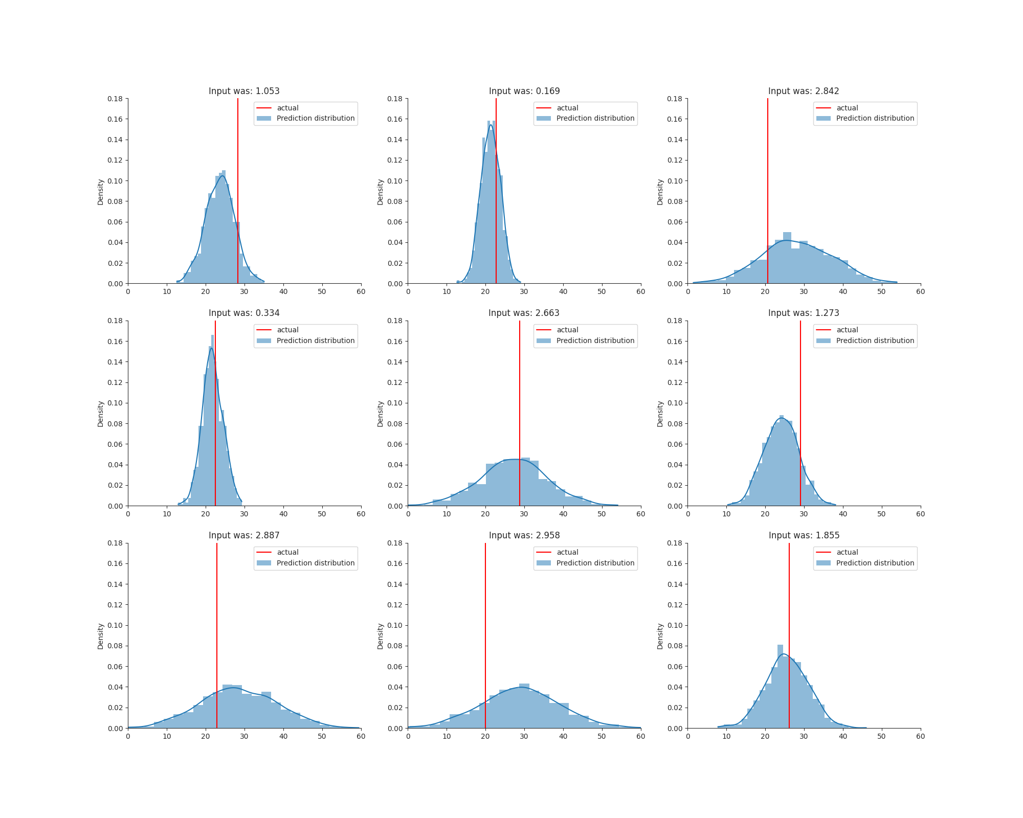
Approximate predictive posterior distribution

When modelling both types of uncertainty, using our .mc_predict() method, we still need to combine them into a single predictive distribution. Last time, we had to uniformly sample from each CDF (approximated by the quantile predictions). This is because the quantile regression method does not make any distribution assumption. It just “follows the data”. This time we’ve assumed our predicted distribution was a normal distribution. This means that all our (Monte Carlo Dropout) samples are normal distributions. This allows us to average all our sampled $\mu$s and $\sigma$s which makes the addition of epistemic uncertainty a lot less computationally heavy.

Discussion

So there it is! Another way of predicting multiple types of uncertainty. Again, we used a toy dataset which only contained one feature to predict $y$. Therefore, the dropout rate had a big impact on the uncertainty and training process. Something that I would like to do next is using this model on a more real life dataset and evaluating the uncertainty. Then we are able to compare different methods. How well do these approaches perform agains eachother, and against a full baysian approach?

References

[1] https://en.wikipedia.org/wiki/Normal_distribution